

Data pipelines can break for a million different reasons, but how can we ensure that data quality issues are identified and addressed in real time—at scale? Sometimes, all it takes is a bit of SQL, some precision and recall, and a holistic approach to data observability.
In this article , we walk through how you can create your own data observability monitors from scratch and leverage basic principles of machine learning to apply them at scale across your data pipelines.
As companies rely on more and more data to power increasingly complex pipelines, it’s imperative that this data is reliable, accurate, and trustworthy. When data breaks—whether from schema changes, null values, duplication, or otherwise—we need to know, and fast. A stale table or erroneous metric, left unchecked, could have negative repercussions for your business down the line.
If you’re a data professional, you may be find yourself asking the following questions time and again when trying to understand the health of your data:
- Is the data up to date?
- Is the data complete?
- Are fields within expected ranges?
- Is the null rate higher or lower than it should be?
- Has the schema changed?
To answer these questions, we can take a page from the software engineer’s playbook: data observability. Data engineers define data observability as an organization’s ability to answer these questions and assess the health of their data ecosystem. Reflecting key variables of data health, the five pillars of data observability are:
- Freshness: is my data up to date? Are there gaps in time where my data has not been updated?
- Distribution: how healthy is my data at the field-level? Is my data within expected ranges?
- Volume: is my data intake meeting expected thresholds?
- Schema: has the formal structure of my data management system changed?
- Lineage: if some of my data is down, what is affected upstream and downstream? How do my data sources depend on one another?
In this article series, we pull back the curtain to investigate what data observability looks like in the code, and in this final installment, we’ll take a step back and think about what makes a good data quality monitor in general. Maybe you’ve read Parts I and II and are thinking to yourself, “these are fun exercises, but how can we actually go about applying the concepts in my real production environment?”
At a high level, machine learning is instrumental for data observability at scale. Detectors outfitted with machine learning can apply more flexibly to larger numbers of tables, eliminating the need for manual checks and rules (as discussed in Parts I and II) as your data warehouse grows. Also, machine learning detectors can learn and adapt to data in real-time, and capture complicated seasonal patterns that would be otherwise invisible to human eyes.
Let’s dive in—no prior machine learning experience required.
Our data environment
This tutorial is based on Exercise 4 of our O’Reilly course, Managing Data Downtime. You’re welcome to try out these exercises on your own using a Jupyter Notebook and SQL.
As you may recall from Parts I and II, we’re working with mock astronomical data about habitable exoplanets. There’s unfortunately nothing real about this data — it was fabricated for pedagogical purposes — but you can pretend it’s streaming direct from Perseverance if you’d like.
We generated the dataset with Python, modeling data and anomalies off of real incidents we’ve come across in production environments. (This dataset is entirely free to use, and the utils folder in the repository contains the code that generated the data).
For this exercise, we’re using SQLite 3.32.3, which should make the database accessible from either the command prompt or SQL files with minimal setup. The concepts extend to really any query language, and these implementations can be extended to MySQL, Snowflake, and other database environments with minimal changes.
In this article, we’re going to restrict our attention to the EXOPLANETS table:

Note that EXOPLANETS is configured to manually track an important piece of metadata — the date_added column — which records the date our system discovered the planet and added it automatically to our databases. In Part I, we used a simple SQL query to visualize the number of new entries added per day:

This query yields data that looks like this:


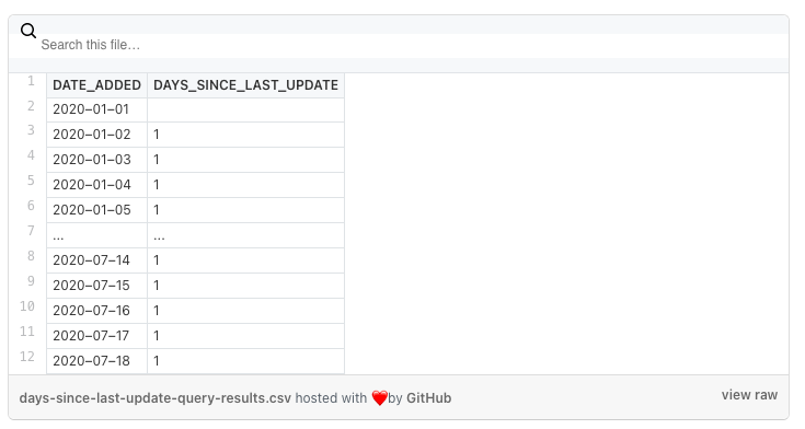
In words, the EXOPLANETS table routinely updates with around 100 entries per day, but goes “offline” on some days when no data is entered. We introduced a metric called DAYS_SINCE_LAST_UPDATE to track this aspect of the table:

The results look like this:

With a small modification, we introduced a threshold parameter to our query to create a freshness detector. Our detector returns all dates where the newest data in EXOPLANETS was older than 1 day.


The spikes in this graph represent instances where the EXOPLANETS table was working with old or “stale” data. In some cases, such outages may be standard operating procedure—maybe our telescope was due for maintenance, so no data was recorded over a weekend. In other cases, though, an outage may represent a genuine problem with data collection or transformation—maybe we changed our dates to ISO format, and the job that traditionally pushed new data is now failing. We might have the heuristic that longer outages are worse, but beyond that, how do we guarantee that we only detect the genuine issues in our data?
The short answer: you can’t. Building a perfect predictor is impossible (for any interesting prediction problem, anyway). But, we can use some concepts from machine learning to frame the problem in a more structured way, and as a result, deliver data observability and trust at scale.
Improving alerting with machine learning
Whenever we alert about a broken data pipeline, we have to question whether the alert was accurate. Does the alert indicate a genuine problem? We might be worried about two scenarios:
- An alert was issued, but there was no genuine issue. We’ve wasted the user’s time responding to the alert.
- There was a genuine issue, but no alert was issued. We’ve let a real problem go undetected.
These two scenarios are described as false positives (predicted anomalous, actually OK) and false negatives (predicted OK, actually anomalous), and we want to avoid them. Issuing a false positive is like crying wolf—we sounded the alarm, but all was ok. Likewise, issuing a false negative is like sleeping on guard duty—something was wrong, but we didn’t do anything.
Our goal is to avoid these circumstances as much as possible, and focus on maximizing true positives (predicted anomalous, actually a problem) and true negatives (predicted OK, actually OK).
Precision and recall
So, we want a good detection scheme to minimize both False Positives and False Negatives. In machine learning practice, it’s more common to think about related but more insightful terms, precision and recall:


Precision, generally, tells us how often we’re right when we issue an alert. Models with good precision output believable alerts, since their high precision guarantees that they cry wolf very infrequently.
Recall, generally, tells us how many issues we actually alert for. Models with good recall are dependable, since their high recall guarantees that they rarely sleep on the job.
Extending our metaphor, a model with good precision is a model that rarely cries wolf—when it issues an alert, you had better believe it. Likewise, a model with good recall is like a good guard dog—you can rest assured that this model will catch all genuine problems.
Balancing precision and recall
The problem, of course, is that you can’t have the best of both worlds. Notice that there’s an explicit tradeoff between these two. How do we get perfect precision? Simple: alert for nothing—sleeping on duty all the time—forcing us to have a False Positive rate of 0%. The problem? Recall will be horrible, since our False Negative rate will be huge.
Likewise, how do we get perfect recall? Also simple: alert for everything—crying wolf at every opportunity—forcing a False Negative rate of 0%. The issue, as expected, is that our False Positive rate will suffer, affecting precision.
Solution: a singular objective
Our world of data is run by quantifiable objectives, and in most cases we’ll want a singular objective to optimize, not two. We can combine both precision and recall into a single metric called an F-score:

F_beta is called a weighted F-score, since different values for beta weigh precision and recall differently in the calculation. In general, an F_beta score says, “I consider recall to be beta times as important as precision.”
When beta = 1, the equation values each equally. Set beta > 1, and recall will be more important for a higher score. In other words, beta > 1 says, “I care more about catching all anomalies than occasionally causing a false alarm.” Likewise, set beta < 1, and precision will be more important. beta < 1 says, “I care more about my alarms being genuine than about catching every real issue.”
Detecting freshness incidents
With our new vocabulary in hand, let’s return to the task of detecting freshness incidents in the EXOPLANETS table. We’re using a simple prediction algorithm, since we turned our query into a detector by setting one model parameter X. Our algorithm says, “Any outage longer than X days is an anomaly, and we will issue an alert for it.” Even in a case as simple as this, precision, recall, and F-scores can help us!
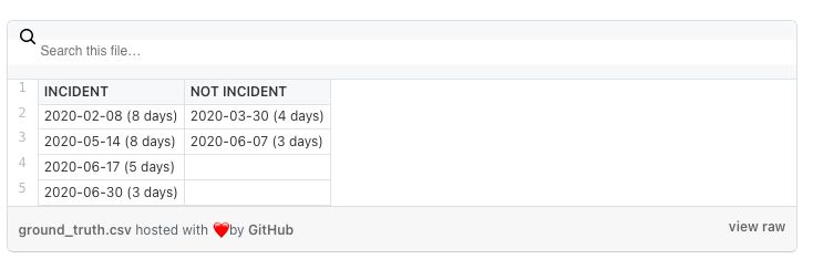
To showcase, we took the freshness outages in EXOPLANETS and assigned ground truth labels encoding whether each outage is a genuine incident or not. It’s impossible to calculate a model’s accuracy without some kind of ground truth, so it’s always helpful to think about how you’d generate these for your use case. Recall that there are a total of 6 outages lasting for more than 1 day in the EXOPLANETS table:

Let’s say, arbitrarily, that the incidents on 2020-02-08 and 2020-05-14 are genuine. Each is 8 days long, so it makes sense that they’d be problematic. On the flip side, suppose that the outages on 2020-03-30 and 2020-06-07 are not actual incidents. These outages are 4 and 3 days long, respectively, so this is not outlandish. Finally, let the outages on 2020-06-17 and 2020-06-30, at 5 and 3 days respectively, also be genuine incidents.
Having chosen our ground truth in this way, we see that longer outages are more likely to be actual issues, but there’s no guarantee. This weak correlation will make a good model effective, but imperfect, just as it would be in more complex, real use cases.
Now, suppose we begin by setting our threshold to 3 days—in words, “every outage longer than 3 days is an anomaly.” This means we correctly detect anomalies on 2020-02-08, 2020-05-14, and 2020-06-17, so we have 3 true positives. But, we unfortunately detected 2020-03-30 as an incident when it isn’t one, so we have 1 false positive. 3 true positives / (3 true positives + 1 false positive) means our precision is 0.75. Also, we failed to detect 2020-06-30 as an incident, meaning we have 1 false negative. 3 true positives / (3 true positives + 1 false negative) means our recall is also 0.75. F_1-score, which is given by the formula.
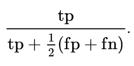
means that our F_1-score is also 0.75. Not bad!
Now, let’s assume we set the threshold higher, at 5 days. Now, we detect only 2020-02-08 and 2020-05-14, the longest outages. These turn out to both be genuine incidents, so we have no false positives, meaning our precision is 1—perfect! But note that we fail to detect other genuine anomalies, 2020-06-17 and 2020-06-30, meaning we have 2 false negatives. 2 true positives / (2 true positives + 2 false negatives) means our recall is 0.5, worse than before. It makes sense that our recall suffered, because we chose a more conservative classifier with a higher threshold. Our F_1-score can again be calculated with the formula above, and turns out to be 0.667.
If we plot our precision, recall, and F_1 in terms of the threshold we set, we see some important patterns. First, aggressive detectors with low thresholds have the best recall, since they’re quicker to alert and thus catch more genuine issues. On the other hand, more passive detectors have better precision, since they only alert for the worst anomalies that are more likely to be genuine. The F_1 score peaks somewhere between these two extremes—in this case, at a threshold of 4 days. Finding the sweet spot is key!

Finally, let’s look at one last comparison. Notice that we’ve only looked at the F_1 score, which weighs precision and recall equally. What happens when we look at other values of beta?

Recall that a general F_beta says “recall is beta times as important as precision.” Thus, we should expect that F_2 is higher than F_1 when recall is prioritized—which is exactly what we see at thresholds less than 4. At the same time, the F_0.5 score is higher for larger thresholds, showing more allowance for conservative classifiers with greater precision.
Data observability at scale with machine learning
We’ve taken a quick safari through machine learning concepts. Now, how can these concepts help us apply detectors to our production environments? The key lies in understanding that there’s no perfect classifier for any anomaly detection problem. There is always a tradeoff between false positives and false negatives, or equally precision and recall. You have to ask yourself, “how do I weigh the tradeoff between these two? What determines the ‘sweet spot’ for my model parameters?” Choosing an F_beta score to optimize will implicitly decide how you weigh these occurrences, and thereby what matters most in your classification problem.
Also, remember that any discussion of model accuracy isn’t complete without some sort of ground truth to compare with the model’s predictions. You need to know what makes a good classification before you know that you have one.
Here’s wishing you no data downtime!
–
Authors: Ryan Kearns and Barr Moses.

